Naïve Math: the Mendocino motor and Earnshaw's theorem
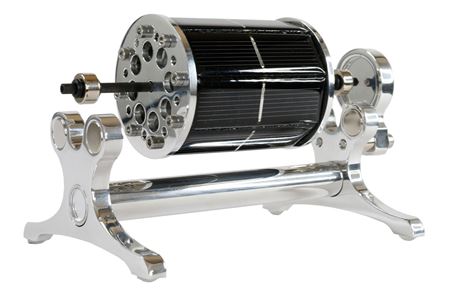
I was surfing the Internet the other day and a rather curious thing caught my mind: the Mendocino motor. It«s an extremely low-friction bearing rotor: the original one had a glass cylinder hanging on two needles, but the modern ones use magnetic suspension. It«s a brushless engine: the rotor has solar batteries attached to it, which generate current for the coils wrapped around the rotor. The rotor spins in a fixed magnetic field, the solar batteries getting exposed to the light source one after the other. It«s a rather elegant solution that«s very possible to recreate at home.
Here«s the video that explains how it works (in Russian):
But this video had another curiosity even stronger than the engine itself. In the video description Dmitry Korzhevsky writes: «You CAN«T replace the side support with a magnet! Don«t ask me about this anymore!»
DIsclaimer: I«m not a physics expert and may be very wrong in some things, so corrections are welcome.
Let«s discuss once again how the rotor«s magnetic suspension system works. If we take two magnets, then the potential isoline looks like this, depending on distance between the magnets:
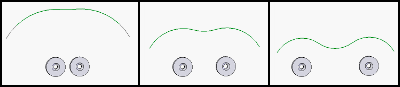
So, we put two fixed magnets on a stator. The magnet placed on the rotor«s axis won«t want to move sideways, since the potential isoline has a certain local minimum point. Instead, it would want to pop out along the rotor«s axis. We make two of these systems and in the end, the rotor«s axis is stable radially, but is unstable laterally. We fix this by tipping the rotor against a glass wall and voila — we have a low-friction bearing.
But the glass wall is a bit… not aesthetically pleasing, isn«t it? It«s only logical we would want to suspend the rotor in the air completely, with no mechanical crutches like this. And evidently, Dmitry was bombarded with the same question as well, which is why he had to note right in the description that it«s impossible. And I bet Dmitry is not the only one who got tired of this.
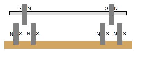
Let us see this, I quote:
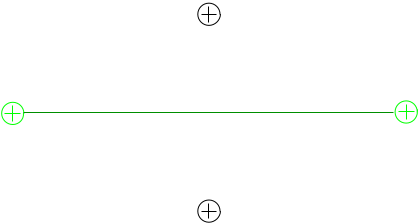
What would happen if the base magnets were spaced and oriented like in this drawing? Would it give it stability in the axial plane, and do away with the mirror requirement?
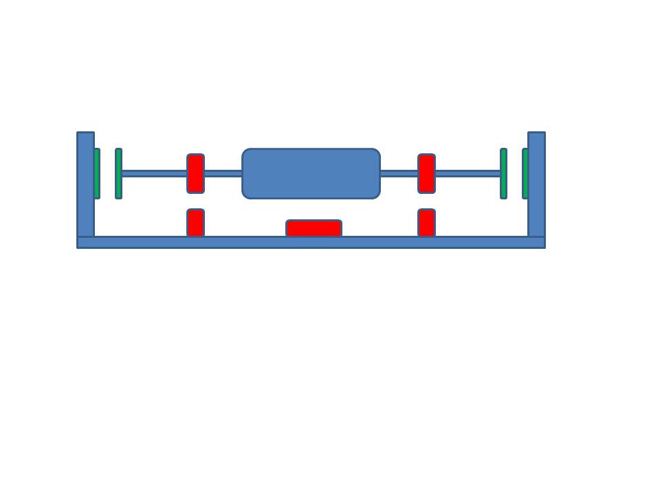
Or here, I quote:
On a Mendocino Motor why does one side float free while the other has a tip to a wall? I know the question might sound trivial but I have worked up the idea why not use the same magnets used to levitate as a counter force on both sides of the shaft? I attached a very rough jpg of what I mean. the green magnets at the end of the shafts is what im referring to. is there some theory or law preventing this?
We can see that a lot of people around the world want to get rid of this unseemly mechanical part. I wasn«t paying much attention back in my schooldays, so it wasn«t at all obvious to me why a completely stable magnetic suspension system was infeasible. One day at lunch I asked that question to my supervisor, a world-famous scientist (in applied mathematics, not physics): «Why is it impossible?». And you know what, he didn«t know it either!
The forums posted above also didn«t provide a proper answer to that question. Best-case, someone referred to something called Earnshaw’s theorem, which doesn«t lend itself to understanding at first glance. It states that: a collection of point charges cannot be maintained in a stable stationary equilibrium configuration solely by the electrostatic interaction of the charges. Did you get it? I certainly didn«t. Let«s say I can accept the fact we«re talking about charges and not magnets. Then what?
When I can«t wrap my head around something, I tend to draw it. Let«s illustrate this in 2D, for simplicity. Imagine four fixed charges, placed in a square pattern, plus a free charge in the center. Like this:
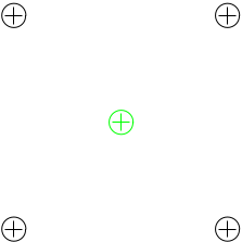
Isn«t the free charge in equilibrium, then? No matter where it moves, it gets closer to one of the fixed charges, which increases the push force! Let«s try to draw a map of a free charge«s potential energy. I missed a lot of physics classes in school, so my repository of knowledge there is Wikipedia. So, if you only have one fixed charge, then it creates electrostatic potential in the field surrounding it:
The equation for electrostatic potential (or Coulomb potential) of a point charge in a vacuum:

In all my thought experiments all coefficients are either 0 or 1. So the q charge is 1, and the unknown k is also 1. That means that one fixed charge creates potential energy measured as 1/r, where r is the distance to the charge.
In our case, the potential energy of the free charge within the fixed charge«s field also equals 1/r. (to be fair, the energy equals k*q1*q2/r, but we pick the coefficients to make calculations easier). For multiple charges we simply add up all potentials.
Let«s draw a map of potential energy of our free charge. I use sage for this:
var('x,y')

def unit_potential(a,b,x,y): return 1/(sqrt((x-a)^2 + (y-b)^2))
def system_potential(x,y): return unit_potential(1,1,x,y)+unit_potential(-1,1,x,y)+unit_potential(1,-1,x,y)+unit_potential(-1,-1,x,y)

contour_plot(system_potential(x,y), (x, -2, 2), (y, -2, 2), cmap='hsv', contours=30, region=5-system_potential(x,y), figsize=12, colorbar=True)
There«s our map. White (punctured) points is where the potential energy goes infinite:
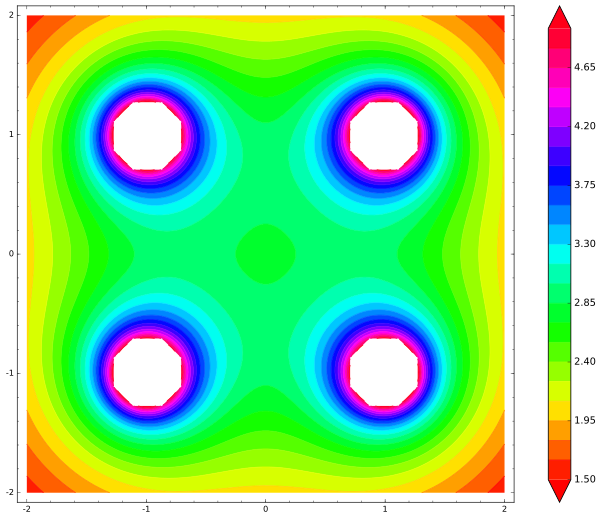
We clearly see the local minimum of energy in the center. Wherever the center charge wants to move, the energy will increase, so small disturbances will force it back to the center — the point of stable equilibrium. Was Earnshaw wrong, then? No, he wasn«t, I just drew the illustration incorrectly. And that«s a common mistake among people who ask that question. Stop for few minutes now and take a guess: what did I miss?
In fact, in this case, the mistake was that in a two-dimensional space, the fixed charge creates potential energy measured as -ln r, where r is the distance to the charge, and not 1/r. Just take my word for the time being and let me correct the equation without explaining a lot. The correct code looks like this:
var('x,y')

def unit_potential(a,b,x,y): return -ln(sqrt((x-a)^2 + (y-b)^2))
def system_potential(x,y): return unit_potential(1,1,x,y)+unit_potential(-1,1,x,y)+unit_potential(1,-1,x,y)+unit_potential(-1,-1,x,y)

contour_plot(system_potential(x,y), (x, -2, 2), (y, -2, 2), cmap='hsv', contours=30, region=5-system_potential(x,y), figsize=12, colorbar=True)
And this is the map it produces:
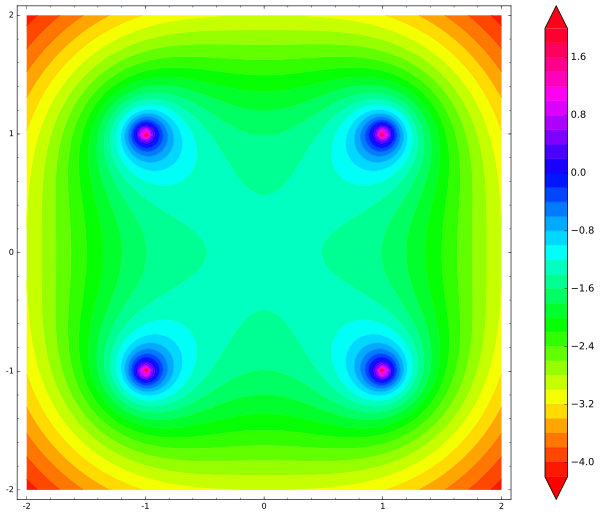
Note that there isn«t a local minimum anywhere. The center is the saddle point, or the point of unstable equilibrium. As soon as the free charge moves even a micron away from the center, it«ll inevitably fly out of the system, accelerating along the way,
Initially, when I realized that my calculations went totally contrary to the Earnshaw theorem, I realized I made a mistake somewhere. It«s easiest to trace my steps from the very beginning. I took a deep breath and went reading about Maxwell’s equations. Again, I wasn«t too good in school: not in grades (these were excellent), but in the amount of knowledge I took away from it. For example, I immediately forgot the Maxwell equations, since in the university and beyond I didn«t have to work with them.
It turns out they«re quite simple, especially if we«re talking about electrostatic laws only! There are four Maxwell equations, one for each of these laws:
- The Gauss law, we«ll need it later. In short, it«s a conservation law: energy can«t be created out of nothing, nor can it be destroyed.
- The Gauss law for magnetic fields, which is essentially the same thing. And we don«t go into magnetic fields yet, since we«re only talking about charged particles. Skip that law.
- The Faraday law: moving magnets create an electric field. That«s interesting, we«ll look at it later.
- The Amper law: moving an electric field creates a magnetic field. Useless for our purposes.
So, these four laws binds two vectors E and B, electric and magnetic fields. These vectors are functions with four arguments (x, y, z, t) and each four arguments gets juxtaposed against one three-dimensional vector. We aren«t that interested into magnetic fields, so let«s take a look at electric fields, or E (x, y, z, t). Don«t forget we«re in the electrostatic realm, so E is constant across time. You can imagine this vector as a river, where at each point we say where and how fast the water goes.
The Faraday law states that a time-constant E field (we«re talking electrostatics there) doesn«t have any curl.
How is electrostatic potential connected to electric fields? Simple: if the E field is curl-less (as it the case there), then we can create u in a way that (going back to the river example), covered by a 1-meter layer of water (at all heights!) and «releasing: it, speed and direction of the water flow would create the E field. Or, in math terms, it«s possible to find a scaling u function, the gradient of which equals the E field.
The Gauss law states: take a small neighborhood. If we didn«t put charges in it deliberately, then the amount of «water» flowing into the neighborhood is equal to the amount flowing out. If we want to sound smart, the E field«s divergence is zero.
Remember: the E field is a derivative of the scaling function u. If its divergence is zero, then it means the laplacian of u is zero. Laplacian is a smart word for the function«s «curve». If we«re talking about one-variable functions, the laplacian is simply the second derivative. In two-variable functions, the laplacian is the sum of two derivatives. If it equals zero, then the curve in one direction should be canceled out by the curve in the other direction. Meaning, crisps can exist:

But the zero-laplacian function doesn«t have local minimums (or maximums), meaning crisps are allowed, but the hills aren«t:

Imagine dipping a (curved) circle of wire into soapy water. The soap film then forms a zero-laplacian surface:
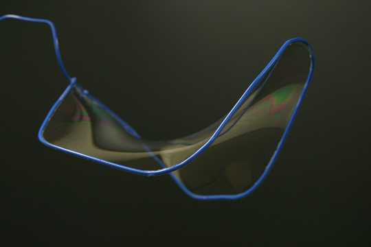
It«ll be the so-called «minimal surface». The soap film tries to be as small as possible, so it«s logical that if it had a certain local maximum, we would have a smaller film by smoothing it out, so there aren«t any. So, electrostatic potential is a sort of a minimal surface that doesn«t have local maximums (as long as we didn«t place charges there deliberately).
The 1/r function has a zero laplacian in three dimensions, but not in two! If we want to draw two-dimensional examples, we would need to solve a Dirichlet problem — for 2D, it«s -ln r.
Using the inverse squares formula in 1- or 2-dimensional space corresponds to restricting the movement of charges along the remaining axes in some other way. In this case, it is obvious that it is possible to make a stable configuration — just take a cardboard tube, put it vertically and put down its magnet. Then it is possible to place there one more magnet which will be in balance — horizontally it is restricted by the tube (i.e. it is in one-dimensional space), and on a vertical force of gravity and repulsion of a magnet are counterbalanced. Earnshaw’s theorem either needs to be applied with the law of inverse squares — but in 3d, or in the space of any dimension, but with the corresponding potential. «Corresponding» means the one obtained from Maxwell’s equations.
So, getting back to our example with one free charged particle. The potential of an electrostatic field doesn«t have local minimums and, as a result, the particle«s potential energy doesn«t have local minimums. So one particle can«t reach stable equilibrium in a static field. Congratulations, we«ve just proved the Earnshaw theorem. But how about more complicated systems? How to apply the theorem there?
Here«s another example that, according to my boss, should«ve disproved the Earnshaw theorem. Let«s fix two charges and create a moving body consisting of a weight-less unstretchable stick with charges at both ends:
Intuitively, if we move the stick slightly to the left or right, then one of the ends would get closer to the fixed charges, which will push it away and return the stick back to the original position. So what«s the catch? Let«s draw a map of electrostatic potential of two fixed charges:
var('x,y')

def unit_potential(a,b,x,y): return -ln(sqrt((x-a)^2 + (y-b)^2))
def system_potential(x,y): return unit_potential(0,1,x,y)+unit_potential(0,-1,x,y)

contour_plot(system_potential(x,y), (x, -2, 2), (y, -2, 2), cmap='hsv', contours=30, figsize=12, colorbar=True)
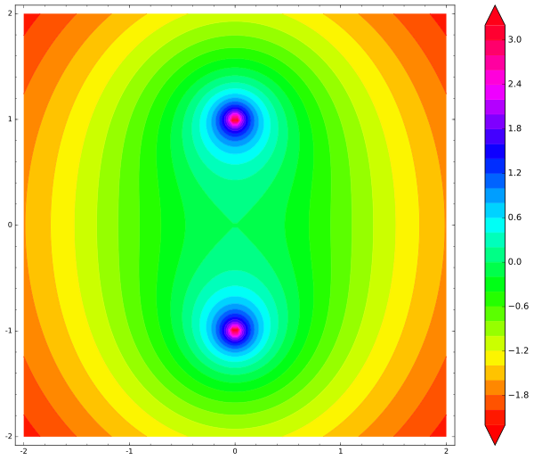
How do we illustrate potential energy of our stick? The stick has three degrees of freedom (two for movement and one for rotation), so the graph would be four-dimensional. Let«s ignore rotation for now and only let the stick move side to side. We fix a point on a stick (for example, its center) and draw the map of the stick«s potential energy for its center. In this case, the total potential energy of the stick is the sum of potential energies of its charges on both ends:
var('x,y')

def unit_potential(a,b,x,y): return -ln(sqrt((x-a)^2 + (y-b)^2))
def system_potential(x,y): return unit_potential(0,1,x,y)+unit_potential(0,-1,x,y)
def energy(x,y): return system_potential(x+2,y)+system_potential(x-2,y)

contour_plot(energy(x,y), (x, -3, 3), (y, -2, 2), cmap='hsv', contours=30, figsize=12, colorbar=True)
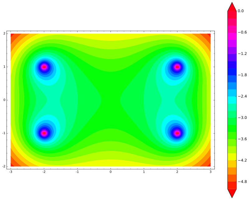
So, the stick«s energy has four peaks (each end can hit each of the two charges). As expected, the stick wouldn«t move horizontally — instead, it would move vertically!
It«s only logical, since how did we get the energy? We added up potential energies of each charge. We know that potential energy of each charge is a zero-laplacian function. Its sum, therefore, also has a zero laplacian. Therefore, the potential energy of any charged body (not just our stick!) can«t have minimums in a static electric field!
Intuitive images of magnetic and electric fields of people who don«t closely work in physics can be misleading. Our brain fools us by making images of energy minimums. Unfortunately, it«s not the case, and creating a Mendocino motor without mechanical support is very difficult, if not impossible.
What loopholes are there to exploit? Earnshaw’s theorem (if we apply it to magnets) only applies to systems of fixed, static magnets.
- We can create a dynamic magnetic field.
- Diamagnetism and superconductors also don«t fall under Earnshaw’s theorem.
- Moving (and specifically, rotating) bodies aren«t discussed there at all, with the levitron being the most famous example.
No, it«s not hopeless. Sure, using any of these loopholes would kill the aesthetics of a Mendocino motor, but the magic of a freely levitating metal thing would trump all of that!
Last note: it was the Earnshaw’s theorem that proved the non-existence of solid matter, therefore disproving the accepted model of an atom, which led to the «planetary» atom model.
